为什么与Yes乐队最相似的歌手是Coda(小田和奏)?
Contents
在网易云音乐中,点入某歌手主页时会有一栏为相似歌手:
Yes是1968年成立的著名前卫摇滚乐队,云音乐中与其相似的列表中有Rush,而后者则是来自加拿大的一支异常出色的前卫摇滚乐队,这对于一个喜爱前卫摇滚的听众来说,当然是一个很不错的推荐。然而,Yes的推荐列表中的第一位是Coda(小田和奏),此君是何许人也,此君并不像Rush、Yes一样是几十年前便成立并在摇滚史上留下浓墨重彩的前卫摇滚音乐人,那云音乐又为何会把此君放在Yes相似列表的第一位呢?
稍微看过Yes歌曲的评论便会知道个中原因,在当今中国大地上Yes这支乐队的歌曲得到曝光,很大程度上是靠《JOJO的奇妙冒险》这部日本动漫中使用了该乐队的音乐,而云音乐里的评论亦均是来自此动漫观光团,而同时这位Coda(小田和奏)的热门歌曲即是该动漫的片头片尾曲,如此便为他们之间的“相似”找到了原因,该观光团必然是既听了Yes的《Roundabout》,又听了此君的作品,因为该动漫的火爆,使得云音乐中那些听过Yes而不看动漫的前卫听众相比因为看该动漫而听Yes的观光团反而成了少数,这直接越过了音乐内容本质,改变了相似列表的值。
看到了上面的例子,很显然这种音乐人之间的相似关联很难仅靠了解音乐的编辑来给出,一方面是音乐人数量巨大,另一个是可能产生关联的维度太多,这便需要寻求集体智慧。
这篇文章使用矩阵分解处理Last.fm 360K数据集,利用海量用户数据来完成音乐人之间相似关系的建立。
加载数据
Last.fm 360K数据集包含了36万users对30万artists的收听情况,文件大小1.6G,共17559530行记录,而在现实的工业应用中,世界著名的音乐软件Spotify在2014年即拥有2400万users与2000万songs。
这种数量级,已经不能像之前介绍item-based CF时直接用numpy生成一个这样shape的用户物品关系矩阵了,稍作计算17559530/(300000*360000)=0.01%后发现此数据集非常稀疏,仅0.01%的位置上有值,毕竟一个user不可能听到很多的artists。scipy提供了几种处理这种稀疏矩阵的方法,可以使矩阵中那些有真实值的位置才占内存,这里使用csr_matrix。
1 | import time |
user count  358868
artist count  292365
plays matrix memory usage: 133 MB.
加载数据后得到稀疏矩阵plays,里面填的值是某user收听某artist的次数,同时写了几个辅助函数,可以通过user_id,artist_name得到在矩阵中相应的值。这里做一个抽样检查,head一下文件第5行会看到’00000c289a1829a808ac09c00daf10bc3c4e223b’这位用户收听’red hot chili peppers’次数为691次。
1 | user1_index = get_row_index_by_user('00000c289a1829a808ac09c00daf10bc3c4e223b') |
00000c289a1829a808ac09c00daf10bc3c4e223b listened red hot chili peppers count: 691.0
矩阵分解理论基础
当然使用基于领域的协同过滤也可以做这个事情,但已经不再合适,首先向量维度越高相互之间计算相似度越慢,更重要的是,决定用户是否喜欢听某歌手的原因可能是多方面的,但绝不是要到30万这个数量级这么多的方面来决定的,这里面并不是一个线性的关系。
矩阵分解是对上述用户物品关系矩阵的降维打击,为user和item各生成一个低维的隐因子,来表达各自的特征: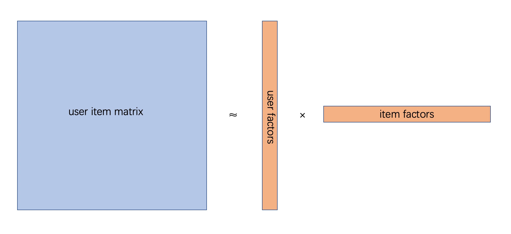
将原矩阵分解成两个矩阵,两矩阵的乘积尽可能与原矩阵相等,越接近越好。对于电影评分这样的显示反馈来讲,损失函数为:
$$
\min _ { x _ { * } , y _ {*} , } \sum _ { u , i } \left( p _ { u i } - x _ { u } ^ { T } y _ { i } \right) ^ { 2 } + \lambda \left( \sum _ { u } \left| x _ { u } \right| ^ { 2 } + \sum _ { i } \left| y _ { i } \right| ^ { 2 } \right)
$$
而对于听音乐这样的隐示反馈,损失函数需要添加一个置信度:
$$
\min _ { x _ { * } , y _ {*} , } \sum _ { u , i } c _ { u i } \left( p _ { u i } - x _ { u } ^ { T } y _ { i } \right) ^ { 2 } + \lambda \left( \sum _ { u } \left| x _ { u } \right| ^ { 2 } + \sum _ { i } \left| y _ { i } \right| ^ { 2 } \right)
$$
其中$c_{ui}$即为置信度,与收听次数有关:
$$
c _ { u i } = 1 + \alpha r _ { u i }
$$
$r_{ui}$为收听次数,$\alpha$为超参数,经验默认值40,$\lambda$为正则化系数,用来防止过拟合。
对上述损失函数的优化方式为ALS的变体Weighted-ALS(加权最小交替二乘法),将item固定,对损失函数求导可得用户向量为:
$$
x _ { u } = \left( Y ^ { T } C ^ { u } Y + \lambda I \right) ^ { - 1 } Y ^ { T } C ^ { u } p ( u )
$$
上式中$Y$为此次计算中被固定的矩阵,$C^{u}$为以用户u的置信度向量生成的对角矩阵,$p(u)$是用户u的收听向量,在用户听过的artist的位置填入1,其他位置填0。
矩阵分解代码
有了上面的公式,很容易使用numpy表示这一计算过程。
1 | def weighted_alternating_least_squares(plays, factors, alpha=40, regularization=0.1, iterations=20): |
依然是数据量的问题,上述代码基本是没法用的。大矩阵各种点乘,空间和时间消费都难以承受。优化方法是利用数学,显然$Y ^ { T } C ^ { u } Y$等于$Y ^ { T } Y + Y ^ { T } \left( C ^ { u } - I \right) Y$,由于当用户u没有收听artist i时,$c_{ui}$为1,使得$\left( C ^ { u } - I \right)$非常稀疏,同时p(u)亦非常稀疏,计算时将矩阵点乘拆开,仅取出有值的部分循环相加即可,如此可极大程度提升计算速度并降低对内存的需求。
implicit的作者在blog中实现了这一过程,里面全是线性代数:
1 | def nonzeros(m, row): |
1 | user_factors, artist_factors = weighted_alternating_least_squares(plays, 50) |
尽管如此,这个分解依然在mac上跑了三个多小时,当然还有更快的方法,implicit库中,作者加了C++代码,可以多线程,并且可以使用GPU加速,10几分钟就可以跑下来360K数据集。
对于置信度的计算方法,论文里还给了另一个效果更好的公式:$c _ { u i } = 1 + \alpha \log \left( 1 + r _ { u i } / \epsilon \right)$,本文提到的第一个置信度计算方式无疑会导致the beatles问题,the beatles太火了大家都听过,导致会出现一些莫名其秒的相似结果,implicit作者推荐使用bm25算法来计算此weight,可以消除这种影响,使结果趋于更加合理的方向。
1 | from implicit.nearest_neighbours import bm25_weight |
100%|██████████| 50.0/50 [20:15<00:00, 23.36s/it]
获取相似artists
生成两矩阵后,表示用户u和artist i的低维稠密向量分别为user_factors[u]与artist_factors[i],它们维数相同。在显示反馈中可用来做用户u对物品i的评分预测,两向量求点积即可;同时,对于两个artists的隐因子向量artist_factors[i1]与artist_factors[i2],依然可以使用余弦相似度公式来计算两者之间的相似度。
问题依然存在,要找到与artist i最相似的几个artists,需要遍历30万隐因子向量计算并排序,这个代价依然是巨大的。既然这里现在有这个问题,那么Spotify肯定早就遇到了,它曾经的推荐组技术带头人Erik Bernhardsson使用C++与Python写了一个用于解决这种近临搜索问题的库annoy,使用起来就是建立一个索引把向量加入进去,搜索时拿着索引去搜很快能得到结果,Approximate Nearest Neighbors,这个Approximate是指在时间与相似程度准确度上进行了取舍。另外相似的工具还有nmslib与facebook开源的faiss。
1 | from annoy import AnnoyIndex |
1 | def get_similar_artists(artist, n = 20): |
yes similar artists:
 ['yes', 'emerson, lake & palmer', 'genesis', 'rush', 'jethro tull', 'king crimson', 'gentle giant', 'the moody blues', 'the alan parsons project', 'camel', 'kansas', 'david gilmour', 'focus', 'supertramp', 'jeff beck', 'roger waters', 'peter gabriel', 'steely dan', 'marillion', 'van der graaf generator']
----------
the_clash similar artists:
 ['the clash', 'ramones', 'pixies', 'iggy pop', 'david bowie', 'the pogues', 'the specials', 'the smiths', 'the rolling stones', 'the cure', 'the white stripes', 'lou reed', 'violent femmes', 'the velvet underground', 'johnny cash', 'joy division', 'beastie boys', 'the kinks', 'nirvana', 'misfits']
----------
the_smiths similar artists:
 ['the smiths', 'morrissey', 'the cure', 'joy division', 'david bowie', 'pixies', 'echo & the bunnymen', 'the clash', 'the jesus and mary chain', 'pulp', 'interpol', 'the velvet underground', 'sonic youth', 'arcade fire', 'elliott smith', 'radiohead', 'my bloody valentine', 'blur', 'lou reed', 'nick drake']
----------
pink_floyd similar artists:
 ['pink floyd', 'led zeppelin', 'the doors', 'jimi hendrix', 'queen', 'jethro tull', 'the police', 'jefferson airplane', 'the jimi hendrix experience', 'the who', 'creedence clearwater revival', 'the rolling stones', 'nirvana', 'dire straits', 'deep purple', 'genesis', 'santana', 'david gilmour', 'john lennon', 'pearl jam']
----------
blur similar artists:
 ['blur', 'franz ferdinand', 'supergrass', 'pulp', 'the dandy warhols', 'the verve', 'manic street preachers', 'the white stripes', 'oasis', 'the stone roses', 'beck', 'primal scream', 'arctic monkeys', 'the coral', 'kasabian', 'david bowie', 'eels', 'the smiths', 'kaiser chiefs', 'new order']
得到的结果令人欣喜。
yes的相似列表里有king crimson,rush,emerson, lake & palmer,genesis,都是前卫得不行的乐队,在前卫摇滚全家福上很容易找到他们的身影;
the clash的列表中ramones,pixies,iggy pop都是朋克乐队,joy division与the clash都是1976年成立,前者是后朋的先驱,看到the velvet underground真的笑出声,毕竟“每一位朋克、后朋克和先锋流行艺术家在过去的30年中都欠下了‘地下丝绒’乐队一笔灵感的债务,哪怕只是受到了间接的影响。”;
the smiths是上个世纪80年代英国独立摇滚的代表,列表中第一位是主唱莫老师,然后有同时期的joy division,echo & the bunnymen,都是独立摇滚的代表;
pink floyd的列表也不必多说,关键字70年代,同一时期历史评价极高的几支乐队都在推荐之列;
最后看到blur的列表里面有pulp和oasis,就放心了。
参考
《Collaborative Filtering for Implicit Feedback Datasets》
Finding Similar Music using Matrix Factorization
A Gentle Introduction to Recommender Systems with Implicit Feedback
Author: Guerbai
Link: http://guerbai.github.io/2019/02/24/matrix-factorization/
License: 知识共享署名-非商业性使用 4.0 国际许可协议